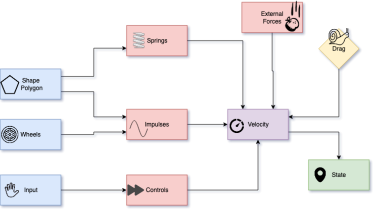
Every object in the original game behaved naturally as a part of the world: it would bounce around when hit, affected by nearby forces, and interacted with the terrain. In this post we are going to describe the mechanics of this model.
Rigid Body
Physics simulation is done using the Newtonian laws as described in a dissertation by Brian Vincent Mirtich (this is the closest reference to the equations I could find, it is possible that there exists a better source of truth). For each body, the following parameters are dynamically tracked and updated:
- position (in world space)
- orientation (in world space)
- linear velocity (in local space)
- angular velocity (in local space)
These parameters are updated regularly with regards to the forces, impulses, time segments, and a bunch of constant factors specified either globally or per particular model. At the high level, each simulation step is done with the following steps:

Impulses
First, we consider all collisions and pushes from another objects as well as the terrain, in order to have a list of impulses that affect the body. The collision vector is computed as a projection of the current velocity at the collision point, projected onto the direction of the collision:
let point_velocity = linear_velocity + cross(angular_velocity, collision_point);
let collision_vector = SOME_CONSTANTS * collision_direction * dot(point_velocity, collision_direction);
In order to evaluate the impulse, we then compute the local collision matrix:
mat3 calc_collision_matrix_inv(vec3 r, mat3 ji) {
    vec3 a = -r.z * ji[1] + r.y * ji[2];
    vec3 b = r.z * ji[0] - r.x * ji[2];
    vec3 c = -r.y * ji[0] + r.x * ji[1];
    mat3 cm = mat3(
        vec3(1.0, 0.0, 0.0) + a.zxy * r.yzx - a.yzx * r.zxy,
        vec3(0.0, 1.0, 0.0) + b.zxy * r.yzx - b.yzx * r.zxy,
        vec3(0.0, 0.0, 1.0) + c.zxy * r.yzx - c.yzx * r.zxy
    );
    return inverse(cm);
}
Here, r is the point of contact, and ji is an inverted Jacobian matrix that is adjusted for volume and scale. These come from the physics part of the model data as described in the Data Formats. My understanding is that the matrix represents an approximation of the distribution of mass in an object, which makes it react respond differently to collisions coming from different directions.
Once the local collision matrix is computed, the raw impulse can be derived as:
let impulse = calc_collision_matrix_inv(collision_point, jacobian_inv) * collision_vector;
This impulse simply adds to the linear velocity, however the effect on the angular velocity requires re-considering the point of collision as well as the Jacobian matrix:
linear_velocity += impulse;
angular_velocity += jacobian_inv * cross(collision_point, impulse);
Forces
Forces are also tracked separately for translation and rotation. Whenever a force vector affects the body at a particular point, we compute the linear and angular components as follows:
fn apply_force(point, vector) {
	linear_force += vector;
	angular_force += cross(point, vector);
}
First force that is always present is gravity. It’s applied at point (0, 0, z_offset_of_mass_center), which comes from the model parameters.
Interestingly, collisions also affect forces, or more specifically - the spring force. It corresponds to some in-game machinery of a car that puts pressure in all directions and can be activated for a jump. Spring force is applied as the force equation at collision_point with collision_vector.
Finally, local effects like vortexes or artifact abilities may also contribute to the forces.
Before the forces can translate into the velocity change, we need to make sure they are converted into the local space. The application is done as follows:
linear_velocity += time_delta * linear_forces;
angular_velocity += time_delta * jacobian_inv * angular_forces;
So technically a force works the same way as an impulse integrated over time, as if the collision_vector is given (as opposed to being computed), which makes the whole model rather elegant in my eyes. In vange-rs, both paths go through a “raw impulse” representation that is common between forces and impulses:
- for forces, they are pre-multiplied by
time_delta - for impulses, the angular component comes from the
cross(point, vector) - multiplication by
jacobian_invis done only once at the end of the simulation step
Velocity application
Note: this section of the post will be updated once new details emerge.
The way the position and orientation are updated by the velocities is still somewhat unclear to me.
let local_z_scaled = real_z_axis_in_local_space * (car_z_radius * IMPULSE_ROLLING_SCALE);
let r_diff_sign = if most_collisions_come_from_the_bottom { 1.0 } else { -1.0 };
let vs = linear_velocity - r_diff_sign * local_z_scaled.cross(angular_velocity);
position += rotate(orientation, vs) * dt;

let angle = Radians(-dt * length(angular_velocity));
let vel_rot_inv = Quaternion::from_axis_angle(normalize(angular_velocity), angle);
orientation *= inverse(vel_rot_inv);

linear_velocity = rotate(vel_rot_inv, linear_velocity);
angular_velocity = vel_rot_inv * angular_velocity;
The first part is confusing: we are computing a modified velocity vector, based on the Z axis direction, the size of the object, and it major collision direction. This velocity gets multiplied by time, transformed into the world space, and added to the position.
In the second part, we are constructing the inverse of the angular velocity vector as a rotation. It ends up multiplying with the orientation as well as rotating both of the velocities.
Drag
Somewhat aside from all this elegant machinery stays the drag force, which is gets contributions from a number of constants but most importantly - from the magnitude of the velocities:
let linear_drag = LINEAR_DRAG_FREE * pow(LINEAR_DRAG_SPEED, length(linear_velocity));
let angular_drag = ANGULAR_DRAG_FREE * pow(ANGULAR_DRAG_SPEED, length_squared(angular_velocity));
Note: the constants are capitalized for clarity here, they are specified in common.prm file.
At the end of the step (after the position and orientation are updated), the velocities simply get multiplied by a drag, which typically stays within 0.9 to 1.0 range.
Terrain
Remember the collision shapes we described in the Data Formats? These simplified quad-based mesh approximations get intersected with the terrain at each step. How? By just rasterizing them on the terrain and sampling the heights (and metadata) at each intersection point.
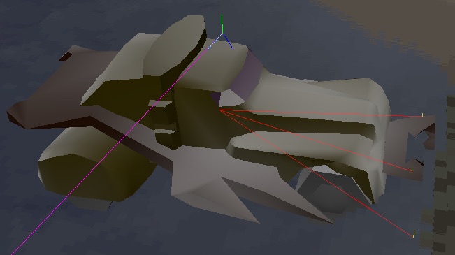
For each collision shape quad, we find the average in the penetration depth (along the Z axis) as well as the point of contact. Then we simply generate an impulse at that point with the vector pointing downwards, following the regular impulse equations. This picture shows the averaged contact points and vectors:

Note: more precisely, the pixels are split into groups for “soft” contacts and “hard” constants, and these averaged contact points are used differently for some logic, like the horizontal wall collisions.
Controls
User-controlled car is also affected by the traction, which is computed separately for each wheel. Each wheel generates an impulse at its position along the rudder vector, following the same impulse equation:
let wheel_collision_direction = vec3(cos(car_rudder), -sin(car_rudder), 0.0);
Jumps are implemented as modification of the linear velocity based on the mass:
fn jump(power) {
	linear_velocity += power * LOCAL_JUMP_DIRECTION / pow(car_mass, 0.3);
}
Simulation Loop
The original game runs the physics step N times per frame with a fixed delta, where N is a constant. In order to adjust for variable frame rate, we introduce a “speed correction factor”, which is a ratio of time_delta / BASE_TIME_DELTA. This factor ends up adjusting various intermediate results during the simulation.
I believe the physics model becomes unstable once we start using the real time_delta for computations. When the original game was released, fixed-framerate games were still a norm, and there wasn’t any expectation of running the game faster than at 20 fps.